
Native and Compact Structured Latents for 3D Generation
The paper proposes O-Voxel, a sparse voxel representation holding both geometry and PBR material, and an SC-VAE with 16x compression so a textured 1024 asset needs about 9.6K tokens. Flow-matching models totaling about 4B parameters generate shape and material from an image, and the authors report gains over baselines in reconstruction and generation experiments.
This paper builds an image-to-3D generator around a new native 3D representation instead of converting meshes into distance fields. The central trade-off is fidelity versus token count: a fully textured 1024-resolution asset is compressed into about 9.6K latent tokens.
Overview
Imagine photographing a toy and getting back a full 3D model, including shiny metal or see-through glass. Many older systems first turn the shape into a blurry "map of distances", which loses thin sheets, hollow insides and sharp edges.
This paper keeps the object as a sparse set of small cubes that exist only where the surface is, and writes both shape and material into each cube. A compressor then shrinks that list so a large generator can work with it quickly.
Objective: generate high-resolution textured 3D assets with arbitrary topology from a single image. The paper (informally TRELLIS.2) argues that existing representations struggle with complex topology and detailed appearance.
Contributions: (1) O-Voxel, a "field-free" sparse voxel structure storing geometry and physically based rendering (PBR) material, including opacity, convertible to and from meshes without optimization or rendering; (2) a Sparse Compression VAE (SC-VAE) with 16x spatial downsampling, giving about 9.6K latent tokens for a fully textured 1024 asset; (3) flow-matching generators with about 4B parameters in total, trained on public 3D datasets.
Why it matters: fewer tokens make large generators affordable; the authors report about 3 s, 17 s and 60 s on an H100 at 512, 1024 and 1536 resolution. The Best Student Paper award is the conference's recognition; the strengths and weaknesses below are a reading of the paper, not part of the award.
TRELLIS.2 combines three parts: a representation that needs no iso-surface field (O-Voxel), a fully sparse-convolutional autoencoder with 16x spatial compression (SC-VAE), and a cascade of three DiT-style flow-matching models for sparse structure, geometry latents and material latents. The introduction claims it far exceeds existing models in geometry and material quality while remaining faster; the evidence is Tables 1 to 3 and qualitative figures, summarised below.
The compactness is the enabling property. With about 9.6K tokens for a 1024 asset, each DiT (about 1.3B parameters) can drop the convolutional packing and skip connections used in the earlier TRELLIS and become a plain encoder-only transformer. The authors list Tsinghua University, Microsoft Research, Microsoft AI and USTC; the first author's work was done during an internship at Microsoft Research. The Best Student Paper status is listed on the official CVPR 2026 award page.
Research Problem
Real 3D models can have holes, double walls, hidden interiors and glass-like parts. Earlier generators often forced every object into one clean closed shape, so they lost detail or needed a lot of computing power.
Recent large 3D generators mostly use iso-surface fields (such as signed distance functions or FlexiCubes) for geometry. The paper says these are intrinsically limited for open surfaces, non-manifold geometry and enclosed interiors. Most systems also concentrate on shape and neglect appearance; the earlier TRELLIS jointly models geometry and appearance but relies on multi-view 2D image features and rendering-only supervision, which the authors say miss complex structures and materials.
Size is the second obstacle. Structured latents (built on sparsity) give accurate geometry but need many tokens; unstructured latents compress strongly but are limited in reconstruction fidelity. Texturing pipelines that generate shape and then multi-view textures also need baking and alignment, which can cause inconsistent appearance.
Formulation: input is one image (training also uses 3D assets); output is a textured mesh with PBR materials. The research question is whether one native representation can describe arbitrary surfaces with materials and still be compact enough to train a billion-parameter generator.
The baselines named by the paper split into three families: unstructured Shape2VecSet-style latents (Dora), sparse-voxel structured latents (Trellis, Direct3D-S2, SparseFlex), and, for generation, systems such as Hi3DGen, Step1X-3D and Hunyuan3D 2.1. Table 1 shows how the families sit on the fidelity versus token trade-off: Dora uses 2.0K to 4.1K tokens but has mesh distances in the hundreds; SparseFlex 1024 reaches 0.3132 with 225K tokens; Trellis has 9.6K tokens but MD 85.07.
Two practical issues sharpen the problem. Evaluating SDFs, flood-filling and iterative optimisation make conversion from meshes slow and force watertightness. And metrics have to capture interior structures, which is why the paper uses mesh distance (point-to-mesh, computed over all surfaces) rather than only a visible-surface Chamfer distance.
Key Idea
Keep everything native and small. Store the object directly as sparse cubes holding shape and material, and squeeze that list hard with an autoencoder designed for it.
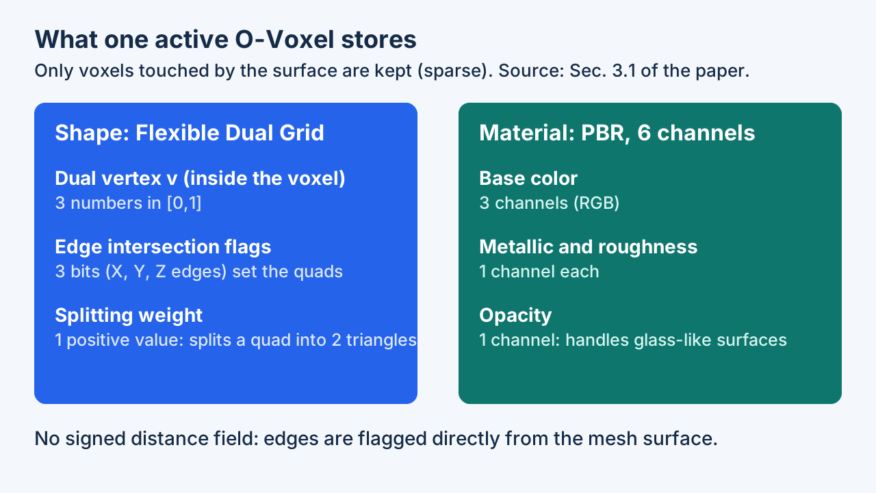
Intuition: a surface only touches a few voxels, so keep only those. Each active voxel stores a dual vertex position, three edge-intersection flags and a splitting weight (shape), plus six material channels: base color (3), metallic, roughness and opacity. Because intersections are read directly from the mesh instead of from sign changes of a field, open, non-manifold and enclosed surfaces are representable.
Difference from prior work: no SDF or other field is used; conversion needs no optimization or rendering ("a few seconds on a single CPU" in the paper, under 10 s on the project page). Opacity lets the representation handle translucent surfaces, which the authors say earlier methods could not.
Second idea: compress aggressively but carefully. SC-VAE adds non-parametric residual shortcuts that move information between space and channels during down- and upsampling, borrowed from DC-AE. Tiny example: when two voxels merge into one coarser voxel, their eight children's features are stacked into channels and averaged, so a parameter-free path carries information alongside the learned convolutions.
Shape follows Dual Contouring, but without a field: the asset's mesh gives edge-intersection flags and Hermite data (points and normals). The dual vertex minimises a quadratic error function, with two extra terms compared with classical DC: $\min_v \sum_i d_{\Pi,i}^2+\lambda_{bound}\sum_j d_{L,j}^2+\lambda_{reg}\|v-\bar q\|^2$. The second term pulls the vertex towards boundary edges (open surfaces); the third keeps it near the mean intersection point and stabilises the solve. Splitting weights follow the flexible-topology rule of FlexiCubes to decide how each quad is split into triangles, and both vertex position and weights can be fine-tuned by rendering losses.
For material, voxel attributes are obtained by projecting voxel centres on triangles, sampling textures and averaging by distance; decoding uses trilinear interpolation. In the SC-VAE the residual shortcut stacks the eight children into channels and averages groups (downsampling), and duplicates channel groups back to children (upsampling). An early-pruning upsampler predicts which of the eight child voxels are active before expansion, saving time and memory, and the residual block replaces two convolutions by one ConvNeXt-style convolution plus a wide point-wise MLP.
Methodology
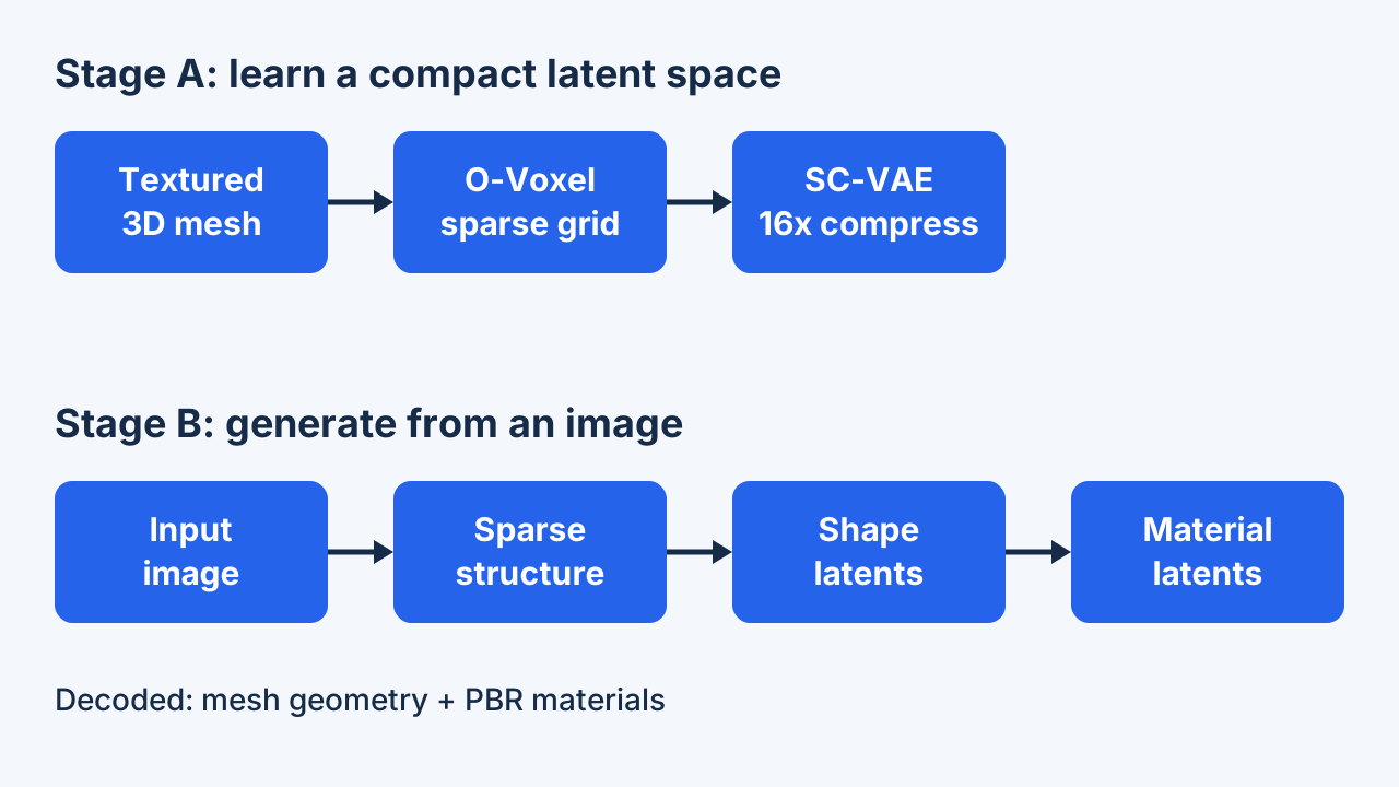
There are two phases. First, teach a compressor to squeeze and rebuild 3D objects. Second, teach a generator to draw objects in the squeezed space step by step: rough layout, then shape detail, then material.
Stage one trains two SC-VAEs, one for shape and one for material; the material VAE is conditioned on the shape VAE's subdivision structure. The network is fully sparse convolutional (a U-shaped VAE, about 800M parameters) rather than a transformer. Training has two phases: 256^3 with direct reconstruction and KL losses, then 512^3 with extra rendering losses on mask, depth, normals and material.
Stage two trains three flow-matching DiTs of about 1.3B parameters each: sparse structure, geometry latents, and material latents conditioned on the image and the generated geometry. Image features come from DINOv3-L. Training is progressive, from 512^3 outputs (32^3 latents) to 1024^3 (64^3 latents).
Data: the SC-VAE uses the Trellis-500K setup filtered to PBR assets (Objaverse-XL, ABO, HSSD); the generators use about 800K assets, augmented with TexVerse. Reported hardware: 16 H100s for SC-VAEs and 32 H100s for DiTs. At inference, a generated O-Voxel can be downsampled and regenerated in a cascade for more resolution or cleaner layouts (Section 4.5).
Losses (Eq. 6 to 8 and Appendix A.3): stage one uses MSE on dual vertices, BCE on edge flags and on the pruning mask, L1 on material and a KL term. Stage two adds rendering terms: for shape, $\|\hat m-m\|_1+10\|\hat d-d\|_1+d_p(\hat n,n)$ on mask, depth and normals; for material, $d_p$ on base color and on the metallic-roughness-alpha map, where $d_p=\|a-b\|_1+0.2\,d_{SSIM}+0.2\,d_{LPIPS}$. Cameras are placed with a shallow near plane so renders slice through surfaces and supervise interiors. Stage one runs at 256^3 and stage two at 512^3; higher resolutions reuse the weights unchanged because the network is fully sparse-convolutional.
Each DiT has width 1536, 30 blocks, 12 heads of dimension 128 and MLP width 8192, with AdaLN-single timestep modulation, RoPE and QK-RMSNorm. The image prompt enters through cross-attention; shape conditioning for the material model is concatenated channel-wise with the input tensor. Training is rectified flow, $x(t)=(1-t)x_0+t\epsilon$ with loss $\|v_\theta(x(t),t)-(\epsilon-x_0)\|_2^2$ and a logit-normal(1,1) timestep sampler as in Trellis; AdamW, learning rate 1e-4, weight decay 0.01, condition drop rate 0.1 for classifier-free guidance. Sparse convolution runs on FlexGEMM, a Triton masked implicit-GEMM backend described in Appendix B (NVIDIA and AMD).
Test-time scaling: max-pool a generated 1024^3 O-Voxel to a 96^3 sparse structure and regenerate geometry to reach 1536^3, or downsample a 512^3 O-Voxel to 64^3 to obtain a cleaner structure for 1024^3. The paper presents this as a controllable compute versus quality trade-off with qualitative evidence (Fig. 8).
Experiments & Results
| Method | Tokens | Downsampling | Dec. (s) | Toys4K MD | Toys4K PSNR | Sketchfab MD | Sketchfab PSNR |
|---|---|---|---|---|---|---|---|
| Trellis | 9.6K | 4x | 0.108 | 85.07 | 30.29 | 49.20 | 24.31 |
| Direct3D-S2 1024 | 17K | 8x | 13.0 | 73.17 | 27.38 | 70.13 | 23.82 |
| SparseFlex 512 | 56K | 4x | 1.22 | 1.303 | 36.56 | 3.221 | 29.46 |
| SparseFlex 1024 | 225K | 4x | 3.21 | 0.3132 | 37.34 | 0.7593 | 32.12 |
| Ours 512 | 2.2K | 16x | 0.077 | 0.0323 | 39.54 | 0.1572 | 31.00 |
| Ours 1024 | 9.6K | 16x | 0.301 | 0.0042 | 43.11 | 0.0170 | 35.26 |
| Method | CLIP | CLIP-N | ULIP-2 | Uni3D | Pref % | Pref-N % |
|---|---|---|---|---|---|---|
| Trellis | 0.876 | 0.748 | 0.470 | 0.414 | 6.40% | 2.82% |
| Hi3DGen | – | 0.753 | 0.395 | 0.373 | – | 6.57% |
| Direct3D-S2 | – | 0.746 | 0.420 | 0.392 | – | 12.2% |
| Step1X-3D | 0.875 | 0.738 | 0.464 | 0.411 | 11.8% | 0.469% |
| Hunyuan3D 2.1 | 0.869 | 0.753 | 0.474 | 0.427 | 13.3% | 7.51% |
| Ours | 0.894 | 0.758 | 0.477 | 0.436 | 66.5% | 69.0% |
| Setting | Tokens | Dec. (ms) | MD | MD F1 | PSNR | LPIPS |
|---|---|---|---|---|---|---|
| SC-VAE f16c32 | 503 | 28.6 | 1.032 | 0.312 | 27.26 | 0.072 |
| f16c32 w/o Residual AE | 503 | 28.7 | 1.747 | 0.268 | 26.73 | 0.081 |
| f16c32 w/o Opt. ResBlock | 503 | 29.6 | 1.198 | 0.285 | 26.67 | 0.083 |
| SC-VAE f32c128 | 118 | 33.9 | 1.405 | 0.273 | 26.65 | 0.081 |
| f32c128 w/o Residual AE | 118 | 34.0 | 7.394 | 0.192 | 25.01 | 0.102 |
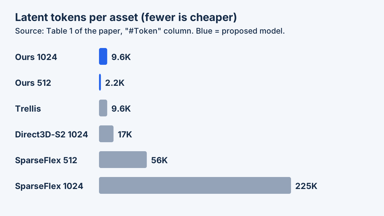
In the authors' tests, the new compressor rebuilt shapes far more accurately than older ones while using far fewer tokens than the strongest older compressor. In a small study, people picked its generated models most often.
Protocols: reconstruction uses Toys4K (473 assets with full PBR maps) and 90 recent Sketchfab "Staff Picks" assets, unseen in training; metrics are mesh distance (MD), visible-surface Chamfer distance, and normal-map PSNR and LPIPS. Generation uses 100 AI-generated image prompts with CLIP, ULIP-2, Uni3D and a user study. Baselines: Dora, Trellis, Direct3D-S2, SparseFlex (reconstruction); Trellis, Hi3DGen, Direct3D-S2, Step1X-3D, Hunyuan3D 2.1 (generation).
Reconstruction (Table 1): at 1024 the model reaches MD 0.0042 on Toys4K against 0.3132 for SparseFlex 1024, using 9.6K tokens instead of 225K and 0.301 s decoding instead of 3.21 s; normal PSNR is 43.11 versus 37.34 dB. The authors state it beats all baselines on every metric of that table. Material reconstruction has no baseline (38.89 dB on PBR maps).
Generation (Table 2): CLIP 0.894 versus 0.876 for Trellis; Uni3D 0.436 versus 0.427 for the best baseline; 66.5% of overall-quality votes in a study of about 40 people. Texturing is compared only qualitatively. Ablation (Table 3): without residual autoencoding, MD rises 69% at 16x and 526% at 32x compression.
Reading Table 1 carefully: the baselines use different downsampling (4x or 8x versus 16x) and token counts, so the table mixes compactness and fidelity. The 512 model (2.2K tokens, MD 0.0323) already beats SparseFlex 1024 on Toys4K MD, normal PSNR and decoding time. On the harder Sketchfab set the margin narrows: MD 0.0170 versus 0.7593 and PSNR 35.26 versus 32.12 dB. Runtimes in Table 1 are on an A100, whereas the 3 s, 17 s and 60 s generation times are on an H100 and come from the introduction and project page, not from a table.
Reading Table 2: the margins in CLIP, CLIP-N and ULIP-2 are small (for example ULIP-2 0.477 versus 0.474), while the user preference is large (66.5% versus 13.3% for the next method). The user study has 202 overall and 213 shape selections from about 40 participants (Table 7), a small pool, on AI-generated prompts. The paper reports no confidence intervals or repeated runs in these tables.
Ablation interpretation (Table 3): the residual shortcut mainly protects strong compression. At f16c32 it improves MD 1.747 to 1.032 and PSNR 26.73 to 27.26; at f32c128 it is the difference between MD 1.405 and 7.394 with only 118 tokens. The optimised block improves quality at near-equal decode time (without it MD 1.198 versus 1.032 and PSNR 26.67 versus 27.26 dB; decode 29.6 versus 28.6 ms), and Table 3 is run at 256^3 on the Sketchfab set only.
Qualitative claims (Fig. 5 to 8, appendix Fig. 11 to 14): thin structures, open leaves, enclosed cockpits and glass or metal materials are shown to be preserved; baselines are described as over-smoothed or artefact-prone, and multi-view texturing as ghosted or seamed. Failure cases are not shown beyond the limitations text.
Limitations
The cubes have a fixed size, so two very close thin layers can blur together. Small holes can appear and are patched afterward. The method also does not know about object parts or meaning.
Reported by the authors
Appendix F lists three limitations. First, representation power is bounded by voxel resolution: if two very close parallel surfaces cross the same voxel, the dual vertex is placed between them and the material is an average, which blurs appearance. Second, reconstructed and generated meshes sometimes contain small holes because a perfectly closed, manifold surface is hard to guarantee from a sparse decoder; standard hole filling mostly fixes them. Third, O-Voxel does not encode part-level or semantic structure.
Future work named by the authors: more stable decoding, part-level segmentation and a graph-based topological structure.
EyeCode analysis (editorial interpretation)
The generation benchmark is only 100 AI-generated prompts and the human study is about 40 people, so broader tests on real photographs would add confidence. The texture comparison is qualitative, and the paper does not show a systematic failure-case study. Reconstruction numbers come from Toys4K (relatively simple objects, as the authors note) plus 90 curated Sketchfab models.
Reported by the authors
The aliasing problem is intrinsic to one dual vertex and one averaged material vector per voxel; structures thinner than the voxel pitch cannot be separated. Hole artefacts are attributed to the sparse decoder's difficulty in guaranteeing closed manifolds at high resolution. Part and semantic structure are absent; the proposed extension is part segmentation plus a graph topology.
EyeCode analysis (editorial interpretation)
Several comparisons are not strictly like-for-like: baselines differ in downsampling factor and token budget, material reconstruction has no baseline, and generation metrics rely on CLIP-family scorers whose gaps are small. Compute is heavy (16 and 32 H100s for training; the README asks for a 24 GB NVIDIA GPU for inference), so independent retraining is costly, although code and weights are public. Whether the compression generalises to very high-frequency textures or to scene-scale content is not tested in the paper.
Key Takeaways
- A good 3D representation should handle holes, insides and materials.
- Compress hard, but add shortcuts so detail survives.
- Generate in stages: outline, shape, then material.
- O-Voxel stores geometry and PBR attributes natively, with no distance field.
- SC-VAE compresses 16x and gives about 9.6K tokens for a textured 1024 asset (Table 1: 225K for SparseFlex 1024).
- Reported results favour the method on Toys4K and Sketchfab reconstruction, on CLIP and Uni3D, and in a user study.
- Stated limits: voxel-resolution aliasing, small holes, no part or semantic structure.
Suggested directions (EyeCode suggestions, not claims from the paper)
- Compare your own sparse autoencoder with and without a parameter-free space-to-channel shortcut.
- Test the released model on real photographs rather than AI-generated prompts.
- Compression is what unlocks scale: the plain DiT, 1.3B per model, is feasible because tokens are about 9.6K at 1024.
- The shortcut-based residual autoencoding is the best-supported component, especially at 32x (MD 7.394 without it versus 1.405).
- Mesh-distance metrics over all surfaces reward interior structure; visible-surface Chamfer alone would not.
- Separate what is quantitative (Tables 1 to 3) from what is visual only (texturing, test-time scaling).
- The award is an official recognition; judgements of wider impact are separate.
Suggested directions (EyeCode suggestions, not claims from the paper)
- Run the released code on a small mesh set and measure token count versus reconstruction error yourself.
- Evaluate hole rates and thin-structure failures on your own assets, since the paper reports them only qualitatively.
- Try the cascade of Section 4.5 and track the quality gain per extra second.
References
- Native and Compact Structured Latents for 3D Generation (arXiv:2512.14692, Tables 1-3, Appendices A-F)
- Native and Compact Structured Latents for 3D Generation (CVF open access, CVPR 2026)
- TRELLIS.2 project page (generation times)
- microsoft/TRELLIS.2 code repository (README, license, roadmap)
- CVPR 2026 Best Papers announcement